death_function <- function(size, mort_prob){
  sampled <- sample(c(0,1), size,replace = TRUE, prob =c(mort_prob, 1- mort_prob))
  return(sampled)
}An introduction
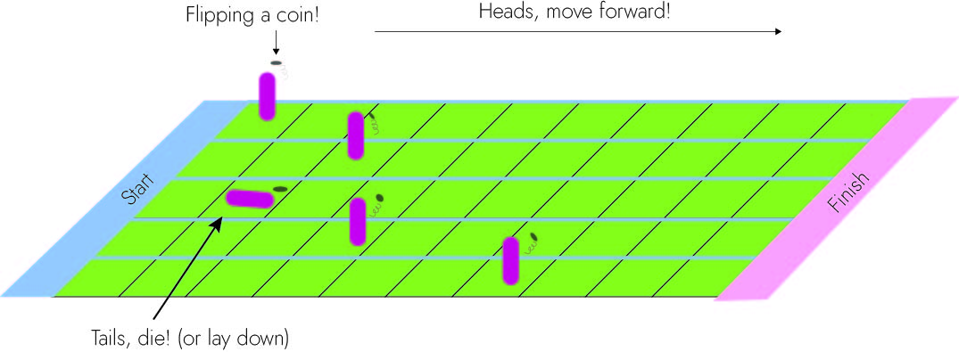
This is a proof-of-concept for a research project I’m developing. Therefore, this is written more for me than for a general audience (sorry!). I can’t give it all away now, but hopefully it’s a taste of what I’m doing. Instead of an ecological question, let’s imagine you are hosting a BBQ and you somehow got a large group of your friends to play a lawn game. Everyone is given a coin and told to flip. If you get heads, you proceed one step. If you get tails, you die (specifically, you just lay down and stay in place). You ‘win’ if you can make it 10 paces away. Here is a schematic below:

But let’s make it more interesting! Let’s assume that the coin can be super biased. Instead of a 50% chance of dying, I manipulate it so that the chance of getting tails can vary from 1% to 100%. Also let’s assume that I introduce some variability. Some friends can only take very small steps and other friends can take larger steps. They somehow need to cumulatively take 10 paces to win, but you can see that there are advantages to those who can take very large steps.
My question is what does it look like at the end of the finish line. Specifically, what are the group of individuals that are able to finish (i.e do they take small steps or big steps?) and what is the timing? How does this differ depending on what kind of mortality coin I give them and what kind of steps I allow them to take?
The simplest code
For the death function, I’m going to use sample until I think a bit more about the gritty mathematics. There is a binary outcome: you survived in this timestep or you perished in this timestep. But we can directly manipulate the probability of mortality.
Now, how do our friends progress through the lawn game. We can give everyone a number (1,2,3) and depending on your number, you can take large steps or very small. You can see that if you are in Group 1, you take smaller steps than individuals in Group 3.
progress_function <- function(id){

  if(id ==1){
  sampled <- runif(1,min =0, max =3)
  }
  else if (id ==2){
  sampled <- runif(1,min = 2,max=5)
  }
  else if (id ==3){
  sampled <- runif(1,min = 5, max =10)
  }
  return(sampled)
}
Now here is the most convoluted code of how the race can begin. A gist of it is that for anyone who has not died, I make them flip the coin. If it’s 0, they stay in place and I record at what time they ‘died’. If it’s a 1, they are still alive where they can make progress to winning. If they accumulate 10 steps, they won and wait while everyone finishes (by either ‘dying’ or ‘winning’).
Code
lawn_race_function <- function(size, mort_prob, progress_time,time_step) {
  full_df <- data.frame(
      current_time = rep(0, size),
      time_event = rep(0, size),
      status = rep(1, size),
      progress = rep(0, size),
       id = rep(c(1, 2, 3), length = size),
       friend_number = seq(1, size))

  survived_subsetted <- full_df [full_df $status == 1 ,]

  i = 0

  while (nrow(full_df [full_df $status == 1 ,]) != 0) {

    i = i + 1
    dead_developed_already_subsetted <- full_df[full_df$status %in% c(0,2),]
    survived_subsetted <- full_df [full_df $status == 1 ,]
    survived_individuals <- nrow(survived_subsetted)
 ###If there are surviving individuals

      survived_subsetted$current_time <- i

      ### Did they die in this time-step?
      survived_subsetted$status <- death_function(survived_individuals, mort_prob)

      if(nrow(  survived_subsetted[survived_subsetted$status == 0, ])!=0){

      survived_subsetted[survived_subsetted$status == 0, ]$time_event <- i

      }
      ### Progressed
      growing_indviduals <- survived_subsetted[survived_subsetted$status == 1, ]

      ###If there are those that will grow
      if(nrow(growing_indviduals) !=0){

      growing_indviduals$progress <- round(growing_indviduals $progress +
                                            time_step*sapply(X = growing_indviduals $id, FUN = progress_function ), 3)

      developed <- growing_indviduals[growing_indviduals$progress >= progress_time, ]

      ###If there are those developed
      if(nrow(developed) != 0){
      growing_indviduals[growing_indviduals$progress >= progress_time, ]$status <- 2
      growing_indviduals[growing_indviduals$status == 2, ]$time_event <- i
      }
      }

      full_df <- rbind(dead_developed_already_subsetted ,
        survived_subsetted[survived_subsetted$status == 0, ],
       growing_indviduals
      )


  }
  return(full_df)
}
The result
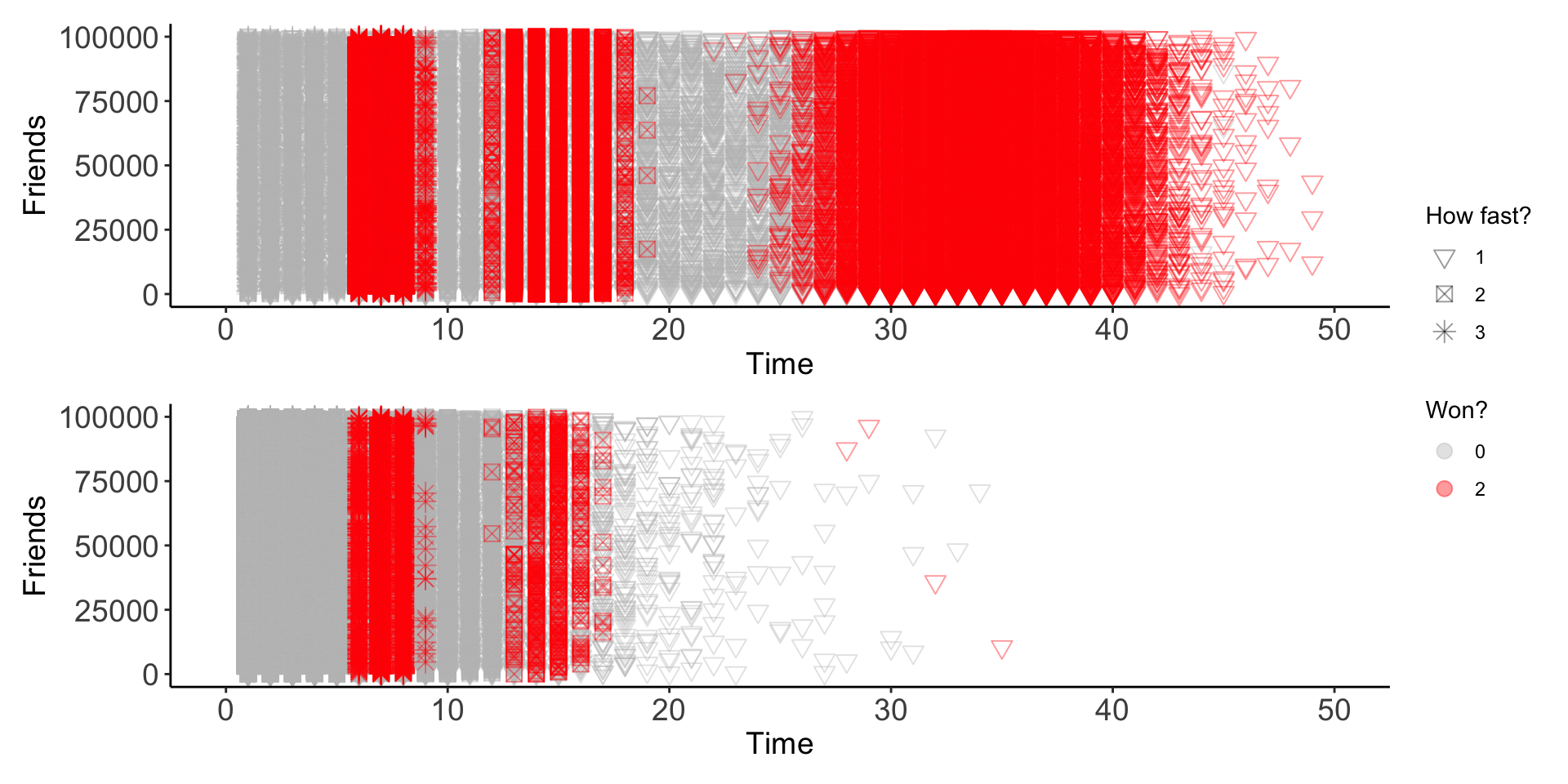
So I set two matches with 100,000 of my friends. The first match, the probability of dying at each time step is 0.001 and you must make 10 steps to win. The second match, the probability of dying at each time step is 0.10 and still you must take 10 steps to win. What does it look like between the two races?
df_lawn_race1<- lawn_race_function(1e5,0.01,10,time_step = 1/5)
df_lawn_race2<- lawn_race_function(1e5,0.40,10,time_step = 1/5)
first_panel / second_panel + plot_layout(guides = 'collect')
So it may be intuitive, but I like having this simulation and figure. When you’re in a race where the chance of mortality is very small, all groups are able to effectively ‘win’. The slower group (Group 3 with the star symbol!) may take a lot longer but eventually they will reach the finish line. However, in the second situation (the bottom graph), with greater chance for mortality, the one who are able to finish the race faster (Group 1) are more likely to win. With each time step.
Let’s take a new perspective
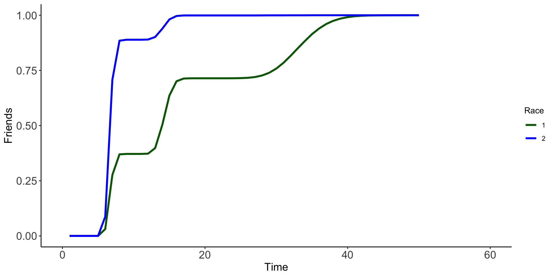
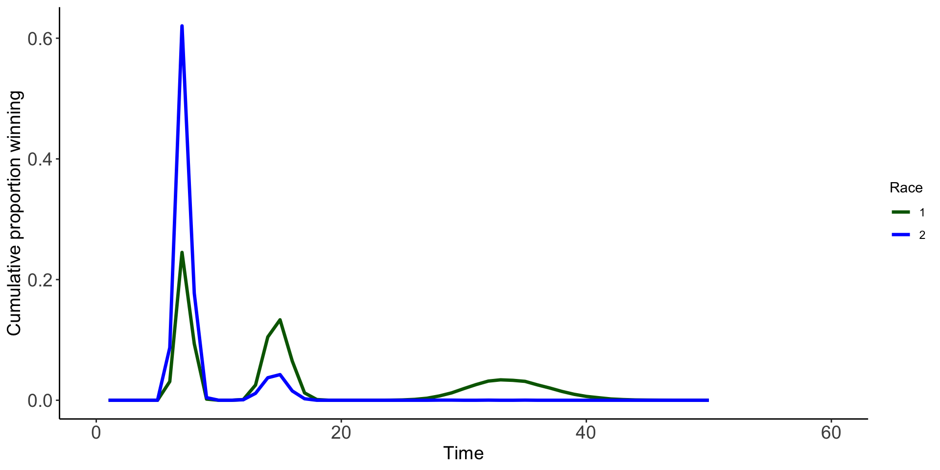
So everyone who won in the game, what does it look as a cumulative proportion over time. The first race (dark green) and second race (blue) are quite different!
Warning: Using `size` aesthetic for lines was deprecated in ggplot2 3.4.0.
ℹ Please use `linewidth` instead.
ggplot(df_full, aes(x = time_event, y= prop, color = as.factor(facet), group = as.factor(facet)))+
 geom_line(size =1.2)+
  xlab("Time")+
  ylab("Cumulative proportion winning")+
  scale_color_manual(name = "Race",values = c(`1` = 'darkgreen', `2` = 'blue'))+
  theme_classic()+
 theme(axis.text = element_text(size = 14),
        axis.title = element_text(size = 14))+xlim(0,60)
Huh… Could there be more variability of individuals winning in the first race?