Lotka-Volterra Competition (Part 2)

Premise

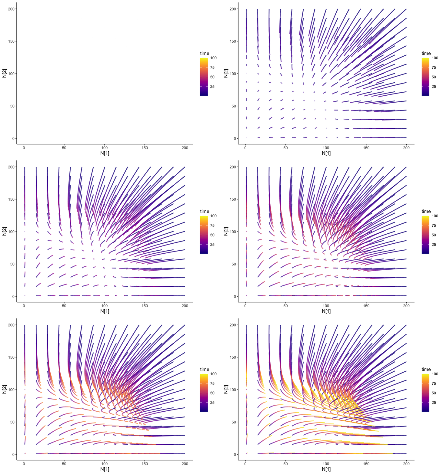
Ok, so from my last blog post on the Lotka-Volterra competition, I was wondering what would happen if I change my competition parameters over time- how would the dynamics change? Just some code for my future self.

library(ggplot2)
library(gganimate)
library(reshape2)
library(viridis)

Again, look at my previous post, but I modified the functions:

# c_df is a data.frame containing the competition coefficients above
# N1_0 is the initial population for N1
# N2_0 is the initial population for N2
# timestep is how long we want ot run it for


LV_func <- function(c_df, N1_0, N2_0, timestep) {
  # Generate a matrix to keep our records
  pop_mat <- matrix(0, nrow = timestep, ncol = 3)
  pop_mat[, 1] <- seq(1, timestep)
  pop_mat[1, 2] <- N1_0 # initial first population
  pop_mat[1, 3] <- N2_0 # initial second population

  ### Competition coefficient
  c_11_v <- c_df["c_11"]
  c_12_v <- c_df["c_12"]
  c_22_v <- c_df["c_22"]
  c_21_v <- c_df["c_21"]

  r <- 0.01 # Intrinsic growth rate is same for all species

  for (t in seq(1, timestep - 1)) {
    c_11 <- c_11_v[t, ]
    c_12 <- c_12_v[t, ]
    c_22 <- c_22_v[t, ]
    c_21 <- c_21_v[t, ]

    N1 <- pop_mat[t, 2] # Get the current population sizes
    N2 <- pop_mat[t, 3]

    N1_change <- r * N1 * (1 - (c_11 * N1 + c_21 * N2))
    N2_change <- r * N2 * (1 - (c_22 * N2 + c_12 * N1))

    pop_mat[t + 1, 2] <- N1 + N1_change
    pop_mat[t + 1, 3] <- N2 + N2_change
  }
  return(pop_mat)
}

timestep <- 100

N12_0 <- expand.grid(
  N1 = seq(1, 200, length = 15),
  N2 = seq(1, 200, length = 15)
)


c_11_vec <- seq(1e-2, 1e-2 * 0.25, length = timestep)

c_df <- data.frame(
  time = seq(1, timestep),
  c_11 = c_11_vec,
  c_22 = rep(1e-2, timestep),
  c_12 = rep(5e-3, timestep),
  c_21 = rep(4e-3, timestep)
)

N12_full <- do.call(
  rbind.data.frame,
  apply(N12_0, 1, function(x) {
    LV_func(
      c_df,
      x["N1"],
      x["N2"],
      timestep = timestep
    )
  },
  simplify = FALSE
  )
)
### Add an id
N12_full$id <- rep(seq(1, nrow(N12_0)), each = timestep)
colnames(N12_full) <- c("time", "N1", "N2", "id")

isocline_N1 <- function(c_df, timestep) {
  ab <- as.numeric(seq(0, 200))

  ### Competition coefficient
  c_11_v <- c_df["c_11"]
  c_21_v <- c_df["c_21"]

  isocline_change_df <- NULL
  for (t in seq(1, timestep)) {
    c_11 <- c_11_v[t, ]
    c_21 <- c_21_v[t, ]

    isocline <- (1 - (c_21 * ab)) / c_11

    isocline_change_df[[t]] <- cbind.data.frame(N1 = isocline, N2 = ab, time = as.numeric(t))
  }
  full <- do.call(rbind, isocline_change_df)
  return(full)
}


isocline_N2 <- function(c_df, timestep) {
  ab <- as.numeric(seq(0, 200))

  ### Competition coefficient
  c_22_v <- c_df["c_22"]
  c_12_v <- c_df["c_12"]

  isocline_change_df <- NULL
  for (t in seq(1, timestep)) {
    c_22 <- c_22_v[t, ]
    c_12 <- c_12_v[t, ]

    isocline <- (1 - (c_12 * ab)) / c_22

    isocline_change_df[[t]] <- cbind.data.frame(N1 = ab, N2 = isocline, time = as.numeric(t))
  }
  full <- do.call(rbind, isocline_change_df)
  return(full)
}

isocline1 <- isocline_N1(c_df, timestep)
isocline2 <- isocline_N2(c_df, timestep)

That is super-neato!

slate + geom_path(
  data = N12_full,
  aes(x = N1, y = N2, group = id, color = time), size = 0.9, alpha = 0.8
) +
  transition_reveal(time) +
  theme_classic() +
  scale_color_viridis(option = "plasma") +
  ease_aes("cubic-in-out")